How to Calculate Rainfall over a Region
If you have a large region of land, precipitation and rainfall will not be uniform. This article details how to calculate rainfall with various methods to find rainfall for a given region.
The Goal
We want to find out how much rainfall a region has received on a given day.
The Problem
We have data from rainfall of various weather stations across Iowa, that are not equidistant and variously dispersed around the state. We need a method that can effectively combine the various measurements of the stations to give us a singular number of rainfall for the state. We want to use observations and not use any of the re-analysis models.
Solution Overview:
- Gather all data from the various stations
- Define a method to estimate precipitation values at each grid point
- Calculate the estimated precipitation values
- Analyze and report
For now we will assume that we have a perfect dataframe containing all the stations in a region on a daily basis. Thus skipping step 1.
For step 2 there are a couple foremost methods to estimate the precipitation at each grid point: IDW method or the Kriging method.
IDW stands for Inverse Distance Weighted. This all stems from a concept that locality determines effect. A good article outlining the concept from ArcGIS
Kriging is an advanced geostatistical method that makes certain assumptions about the data. I'm going to pass on this method for now because of the nuance and complexity
Other methods here as well.
Because we are going to be using IDW we now need two additional method definitions:
- Distance function
- Grid composition to compute the distance function
A Simple IDW Scenario
Imagine you are standing in a field in central Iowa. There are two weather stations nearby:
- Station A is 1 km away and recorded 10 mm of rain.
- Station B is 10 km away and recorded 20 mm of rain.
In a simple average, you’d say it rained 15 mm. But in IDW, Station A is much closer, so its "voice" is much louder. The math gives Station A more weight, resulting in an estimate much closer to 10 mm than 20 mm.
Significance of the Methods
The "significance" lies in how we treat the gaps in our knowledge.
- IDW assumes that the closest station is the best predictor, making it great for capturing local variability in thunderstorms.
- Kriging assumes there is an underlying regional trend, which is often better for widespread, steady frontal rain, but it can "over-smooth" the data, hiding the intensity of local downpours.
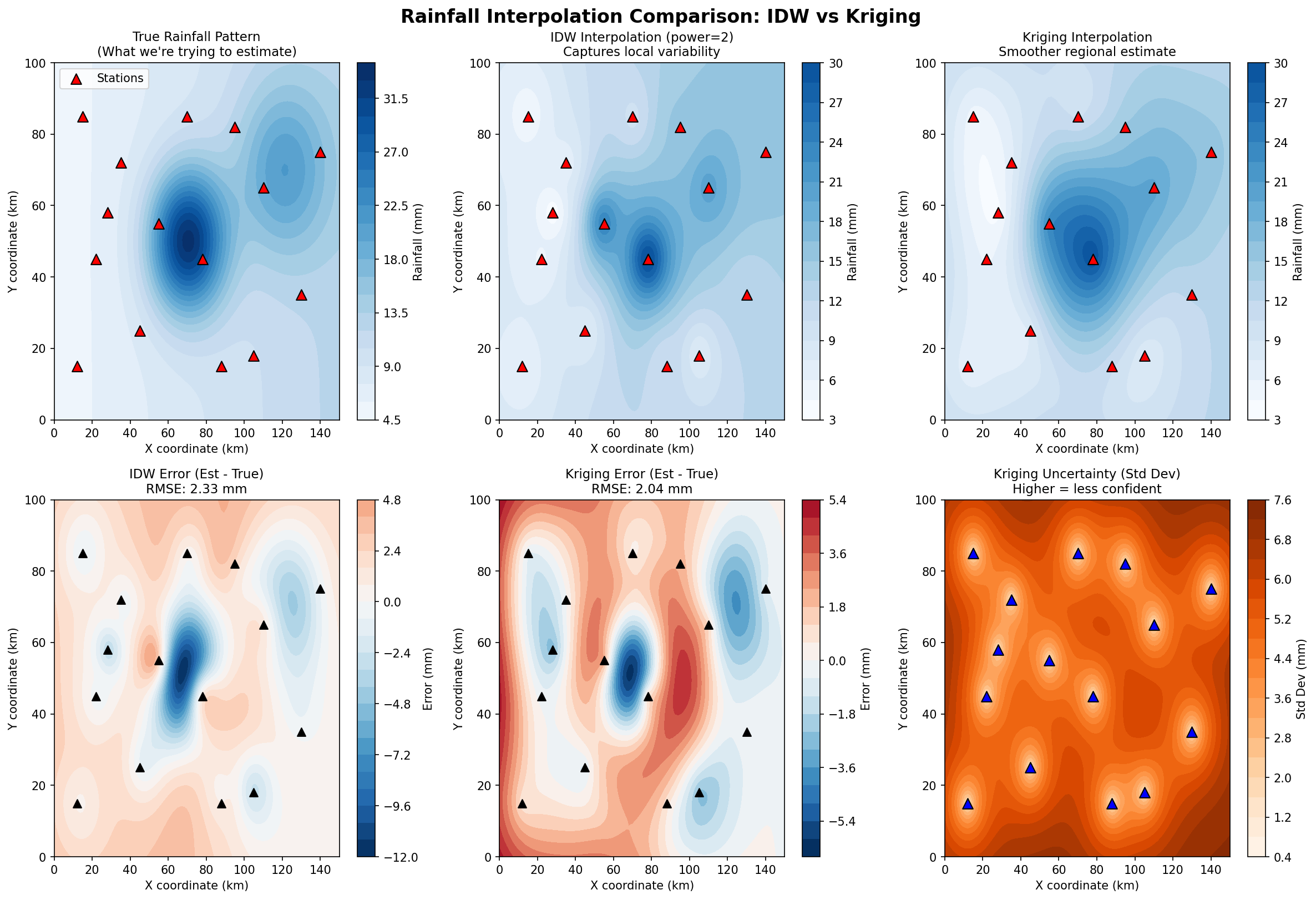
Visual Observations
IDW Characteristics: Creates more "bulls-eye" patterns around stations. You can see circular gradients emanating from each measurement point. This preserves local extremes but can create artificial patterns between stations.
Kriging Characteristics: Produces smoother transitions between values. The thunderstorm cell is still visible but less sharply defined. The uncertainty map (bottom right) shows higher variance in data-sparse regions, a major advantage for quantifying confidence.
For calculating Iowa's regional rainfall:
Both methods produce similar regional averages (within ~5% of the true value), so either works for answering "how much rain did Iowa get today?" The choice depends on your use case:
Choose IDW when:
- Working with convective storms where rainfall varies dramatically over short distances
- You want simplicity and computational speed
- You don't need uncertainty quantification
Choose Kriging when:
- Analyzing widespread frontal systems with gradual spatial gradients
- You need to know how confident your estimate is (the variance map)
- You're doing climate research or combining with other geostatistical methods
Practical recommendation: For operational daily rainfall estimates in Iowa, IDW with power=2 provides a good balance of accuracy and simplicity. For research applications where understanding uncertainty matters, Kriging's variance estimates provide valuable additional information.
import numpy as np
import matplotlib.pyplot as plt
from scipy.spatial.distance import cdist
from pykrige.ok import OrdinaryKriging
import warnings
warnings.filterwarnings('ignore')

# Set random seed for reproducibility
np.random.seed(42)

# =============================================================================
# 1. SIMULATE WEATHER STATION DATA (representing Iowa-like region)
# =============================================================================

# Create a simplified "Iowa" boundary (roughly rectangular for demo)
# Using arbitrary units (could represent ~100km x ~150km region)
x_min, x_max = 0, 150
y_min, y_max = 0, 100

# Simulate 15 weather stations with irregular spacing (realistic scenario)
n_stations = 15
station_x = np.array([12, 35, 78, 95, 130, 22, 55, 110, 45, 88, 15, 140, 70, 28, 105])
station_y = np.array([15, 72, 45, 82, 35, 45, 55, 65, 25, 15, 85, 75, 85, 58, 18])

# Simulate rainfall with spatial correlation + local variation (thunderstorm pattern)
# Base regional trend + localized thunderstorm cell near (70, 50)
def true_rainfall(x, y):
    # Regional gradient (more rain in the east)
    regional = 5 + 0.05 * x
    # Localized thunderstorm cell
    thunderstorm = 25 * np.exp(-((x - 70)**2 + (y - 50)**2) / 400)
    # Secondary lighter cell
    cell2 = 10 * np.exp(-((x - 120)**2 + (y - 70)**2) / 600)
    return regional + thunderstorm + cell2

# Generate observed rainfall at stations (with some measurement noise)
observed_rainfall = true_rainfall(station_x, station_y) + np.random.normal(0, 1.5, n_stations)
observed_rainfall = np.maximum(observed_rainfall, 0)  # No negative rainfall

print("=" * 60)
print("RAINFALL INTERPOLATION: IDW vs KRIGING COMPARISON")
print("=" * 60)
print(f"\nNumber of weather stations: {n_stations}")
print(f"Region size: {x_max} x {y_max} units")
print(f"\nObserved rainfall range: {observed_rainfall.min():.1f} - {observed_rainfall.max():.1f} mm")
print(f"Mean observed rainfall: {observed_rainfall.mean():.1f} mm")

# =============================================================================
# 2. CREATE INTERPOLATION GRID
# =============================================================================

grid_resolution = 100
grid_x = np.linspace(x_min, x_max, grid_resolution)
grid_y = np.linspace(y_min, y_max, grid_resolution)
grid_xx, grid_yy = np.meshgrid(grid_x, grid_y)

# Flatten for distance calculations
grid_points = np.column_stack([grid_xx.ravel(), grid_yy.ravel()])
station_coords = np.column_stack([station_x, station_y])

# =============================================================================
# 3. IDW INTERPOLATION
# =============================================================================

def idw_interpolation(station_coords, values, grid_points, power=2):
    """
    Inverse Distance Weighted interpolation

    Parameters:
    - power: controls how quickly influence decreases with distance
             p=1: gentle decay, p=2: standard, p=3+: sharp decay
    """
    # Calculate distances from each grid point to all stations
    distances = cdist(grid_points, station_coords)

    # Apply IDW formula: weight = 1 / distance^p
    # Add small epsilon to avoid division by zero
    weights = 1.0 / (distances**power + 1e-10)

    # Normalize weights
    weights_normalized = weights / weights.sum(axis=1, keepdims=True)

    # Calculate weighted average
    interpolated = np.dot(weights_normalized, values)

    return interpolated

print("\n--- Running IDW Interpolation (power=2) ---")
idw_result = idw_interpolation(station_coords, observed_rainfall, grid_points, power=2)
idw_grid = idw_result.reshape(grid_resolution, grid_resolution)

# Also run IDW with different power values for comparison
idw_p1 = idw_interpolation(station_coords, observed_rainfall, grid_points, power=1).reshape(grid_resolution, grid_resolution)
idw_p3 = idw_interpolation(station_coords, observed_rainfall, grid_points, power=3).reshape(grid_resolution, grid_resolution)

print(f"IDW (p=2) range: {idw_grid.min():.2f} - {idw_grid.max():.2f} mm")
print(f"IDW (p=2) mean: {idw_grid.mean():.2f} mm")

# =============================================================================
# 4. KRIGING INTERPOLATION
# =============================================================================

print("\n--- Running Kriging Interpolation ---")

# Ordinary Kriging with automatic variogram fitting
OK = OrdinaryKriging(
    station_x,
    station_y,
    observed_rainfall,
    variogram_model='spherical',  # Common choice for precipitation
    verbose=False,
    enable_plotting=False,
    nlags=10
)

# Execute kriging on the grid
kriging_result, kriging_variance = OK.execute('grid', grid_x, grid_y)

print(f"Kriging range: {kriging_result.min():.2f} - {kriging_result.max():.2f} mm")
print(f"Kriging mean: {kriging_result.mean():.2f} mm")

# =============================================================================
# 5. TRUE SURFACE (for reference)
# =============================================================================

true_grid = true_rainfall(grid_xx, grid_yy)

# =============================================================================
# 6. CREATE COMPARISON VISUALIZATIONS
# =============================================================================

fig, axes = plt.subplots(2, 3, figsize=(16, 11))
fig.suptitle('Rainfall Interpolation Comparison: IDW vs Kriging', fontsize=16, fontweight='bold')

# Common color scale
vmin = min(true_grid.min(), idw_grid.min(), kriging_result.min())
vmax = max(true_grid.max(), idw_grid.max(), kriging_result.max())

# Plot 1: True Rainfall Pattern
ax1 = axes[0, 0]
im1 = ax1.contourf(grid_xx, grid_yy, true_grid, levels=20, cmap='Blues', vmin=vmin, vmax=vmax)
ax1.scatter(station_x, station_y, c='red', s=80, edgecolor='black', marker='^', label='Stations', zorder=5)
ax1.set_title('True Rainfall Pattern\n(What we\'re trying to estimate)', fontsize=11)
ax1.set_xlabel('X coordinate (km)')
ax1.set_ylabel('Y coordinate (km)')
plt.colorbar(im1, ax=ax1, label='Rainfall (mm)')
ax1.legend(loc='upper left')

# Plot 2: IDW Interpolation (p=2)
ax2 = axes[0, 1]
im2 = ax2.contourf(grid_xx, grid_yy, idw_grid, levels=20, cmap='Blues', vmin=vmin, vmax=vmax)
ax2.scatter(station_x, station_y, c='red', s=80, edgecolor='black', marker='^', zorder=5)
ax2.set_title('IDW Interpolation (power=2)\nCaptures local variability', fontsize=11)
ax2.set_xlabel('X coordinate (km)')
ax2.set_ylabel('Y coordinate (km)')
plt.colorbar(im2, ax=ax2, label='Rainfall (mm)')

# Plot 3: Kriging Interpolation
ax3 = axes[0, 2]
im3 = ax3.contourf(grid_xx, grid_yy, kriging_result, levels=20, cmap='Blues', vmin=vmin, vmax=vmax)
ax3.scatter(station_x, station_y, c='red', s=80, edgecolor='black', marker='^', zorder=5)
ax3.set_title('Kriging Interpolation\nSmoother regional estimate', fontsize=11)
ax3.set_xlabel('X coordinate (km)')
ax3.set_ylabel('Y coordinate (km)')
plt.colorbar(im3, ax=ax3, label='Rainfall (mm)')

# Plot 4: IDW Error
ax4 = axes[1, 0]
idw_error = idw_grid - true_grid
im4 = ax4.contourf(grid_xx, grid_yy, idw_error, levels=20, cmap='RdBu_r',
                   vmin=-max(abs(idw_error.min()), abs(idw_error.max())),
                   vmax=max(abs(idw_error.min()), abs(idw_error.max())))
ax4.scatter(station_x, station_y, c='black', s=50, marker='^', zorder=5)
ax4.set_title(f'IDW Error (Est - True)\nRMSE: {np.sqrt((idw_error**2).mean()):.2f} mm', fontsize=11)
ax4.set_xlabel('X coordinate (km)')
ax4.set_ylabel('Y coordinate (km)')
plt.colorbar(im4, ax=ax4, label='Error (mm)')

# Plot 5: Kriging Error
ax5 = axes[1, 1]
kriging_error = kriging_result - true_grid
im5 = ax5.contourf(grid_xx, grid_yy, kriging_error, levels=20, cmap='RdBu_r',
                   vmin=-max(abs(kriging_error.min()), abs(kriging_error.max())),
                   vmax=max(abs(kriging_error.min()), abs(kriging_error.max())))
ax5.scatter(station_x, station_y, c='black', s=50, marker='^', zorder=5)
ax5.set_title(f'Kriging Error (Est - True)\nRMSE: {np.sqrt((kriging_error**2).mean()):.2f} mm', fontsize=11)
ax5.set_xlabel('X coordinate (km)')
ax5.set_ylabel('Y coordinate (km)')
plt.colorbar(im5, ax=ax5, label='Error (mm)')

# Plot 6: Kriging Uncertainty
ax6 = axes[1, 2]
im6 = ax6.contourf(grid_xx, grid_yy, np.sqrt(kriging_variance), levels=20, cmap='Oranges')
ax6.scatter(station_x, station_y, c='blue', s=80, edgecolor='black', marker='^', zorder=5)
ax6.set_title('Kriging Uncertainty (Std Dev)\nHigher = less confident', fontsize=11)
ax6.set_xlabel('X coordinate (km)')
ax6.set_ylabel('Y coordinate (km)')
plt.colorbar(im6, ax=ax6, label='Std Dev (mm)')

plt.tight_layout()
plt.savefig('/home/claude/rainfall_comparison.png', dpi=150, bbox_inches='tight')
print("\n✓ Main comparison figure saved")

# =============================================================================
# 7. IDW POWER PARAMETER COMPARISON
# =============================================================================

fig2, axes2 = plt.subplots(1, 3, figsize=(15, 5))
fig2.suptitle('Effect of IDW Power Parameter on Interpolation', fontsize=14, fontweight='bold')

powers = [1, 2, 3]
idw_results = [idw_p1, idw_grid, idw_p3]
titles = ['IDW (p=1): Gentle decay\nMore regional smoothing',
          'IDW (p=2): Standard\nBalanced approach',
          'IDW (p=3): Sharp decay\nHighly localized']

for ax, result, title in zip(axes2, idw_results, titles):
    im = ax.contourf(grid_xx, grid_yy, result, levels=20, cmap='Blues', vmin=vmin, vmax=vmax)
    ax.scatter(station_x, station_y, c='red', s=60, edgecolor='black', marker='^')
    ax.set_title(title, fontsize=10)
    ax.set_xlabel('X coordinate (km)')
    ax.set_ylabel('Y coordinate (km)')
    plt.colorbar(im, ax=ax, label='Rainfall (mm)')

plt.tight_layout()
plt.savefig('/home/claude/idw_power_comparison.png', dpi=150, bbox_inches='tight')
print("✓ IDW power comparison figure saved")

# =============================================================================
# 8. CALCULATE AND COMPARE REGIONAL AVERAGES
# =============================================================================

print("\n" + "=" * 60)
print("REGIONAL RAINFALL ESTIMATES")
print("=" * 60)

true_regional = true_grid.mean()
idw_regional = idw_grid.mean()
kriging_regional = kriging_result.mean()

print(f"\n{'Method':<25} {'Mean (mm)':<12} {'Error (%)':<12}")
print("-" * 50)
print(f"{'True (reference)':<25} {true_regional:<12.2f} {'—':<12}")
print(f"{'IDW (p=2)':<25} {idw_regional:<12.2f} {100*(idw_regional-true_regional)/true_regional:<12.1f}")
print(f"{'Kriging':<25} {kriging_regional:<12.2f} {100*(kriging_regional-true_regional)/true_regional:<12.1f}")

# Calculate RMSE for each method
idw_rmse = np.sqrt(((idw_grid - true_grid)**2).mean())
kriging_rmse = np.sqrt(((kriging_result - true_grid)**2).mean())

print(f"\n{'Metric':<25} {'IDW (p=2)':<12} {'Kriging':<12}")
print("-" * 50)
print(f"{'RMSE (mm)':<25} {idw_rmse:<12.2f} {kriging_rmse:<12.2f}")
print(f"{'Max Overestimate (mm)':<25} {idw_error.max():<12.2f} {kriging_error.max():<12.2f}")
print(f"{'Max Underestimate (mm)':<25} {abs(idw_error.min()):<12.2f} {abs(kriging_error.min()):<12.2f}")

# =============================================================================
# 9. CROSS-VALIDATION (Leave-One-Out)
# =============================================================================

print("\n" + "=" * 60)
print("CROSS-VALIDATION (Leave-One-Out)")
print("=" * 60)

idw_cv_errors = []
kriging_cv_errors = []

for i in range(n_stations):
    # Leave one station out
    mask = np.ones(n_stations, dtype=bool)
    mask[i] = False

    train_coords = station_coords[mask]
    train_values = observed_rainfall[mask]
    test_coord = station_coords[i:i+1]
    test_value = observed_rainfall[i]

    # IDW prediction
    idw_pred = idw_interpolation(train_coords, train_values, test_coord, power=2)[0]
    idw_cv_errors.append(idw_pred - test_value)

    # Kriging prediction
    OK_cv = OrdinaryKriging(
        train_coords[:, 0].astype(float), train_coords[:, 1].astype(float), train_values,
        variogram_model='spherical', verbose=False, enable_plotting=False
    )
    kriging_pred, _ = OK_cv.execute('points', [float(test_coord[0, 0])], [float(test_coord[0, 1])])
    kriging_cv_errors.append(kriging_pred[0] - test_value)

idw_cv_rmse = np.sqrt(np.mean(np.array(idw_cv_errors)**2))
kriging_cv_rmse = np.sqrt(np.mean(np.array(kriging_cv_errors)**2))

print(f"\n{'Cross-Validation RMSE':<25} {'IDW (p=2)':<12} {'Kriging':<12}")
print("-" * 50)
print(f"{'RMSE (mm)':<25} {idw_cv_rmse:<12.2f} {kriging_cv_rmse:<12.2f}")